A GUIDE TO STATE OF THE ART OBJECT DETECTION FOR MULTIMODAL NLP

Introduction

If you’re reading this, chances are you’re a computational linguist and chances are you have not had a lot of contact with computer vision. You might even think to yourself “Well yeah, why would I? It has nothing to do with language, does it?” But what if a language model could also rely on visual signals and ground language? This would definitely help in many situations: Take, for example, ambiguous formulations where textual context alone cannot decide whether “Help me into the car!” would refer to an automobile or a train car. As it turns out, people are working very hard on exactly that; combining computer vision with natural language processing (NLP). This is a case of so called Multimodal Learning.

“But why?”

Multimodality is desirable for a number of reasons and use cases.

A discipline that is well known in computational linguistics is the task of question answering: We give a model a text, ask it a question regarding that text and the model will try to answer our question. This task is considered unimodal since the text and the question are represented in the same modality, i.e. written language. Visual question answering is the multimodal version of the same task where we give the model an image instead of a text and ask it a question about that image.

What if we also want to ask the model a series of follow-up questions? Follow-up questions typically depend on the previous questions and responses, just like they would in a natural language dialogue. Then we have an extension of the previous task, called visual dialogue.

Instead of asking our model a question and having it answer, we might want the model to be more productive and actively describe the image using natural language. This task goes by the name of image captioning.

If we already have an image and a phrase describing it and then ask the model to point to the image region that the description phrase is referring to, we’re speaking of phrase grounding.

As you can see, there are many interesting machine learning/AI tasks that deal with multimodality.

Object detection is the computer vision task of locating and classifying objects in an image
and it is already used in multimodality for image captioning [17]. By identifying objects in an image, object detection plays a crucial role in parsing an image as a scene graph (scene graph parsing). These scene graphs describe the image in an abstract and semantic graph that can then be used to generate natural language descriptions of the image.

If we want to look ahead a little further into the future, object detection is attractive for scenarios such as zero shot learning. The goal here would be to be able to locate an object in an image based off of its descriptions, even if the network has never seen such an object before [1][2]. Think of a personal assistant AI that knows what object you mean when you tell it something like “that [adjective] [thing] that kinda looks like [another thing] except [attribute]”.

With this write-up, I’m hoping to provide a crash course in select state-of-the art object detection models. My goal is to provide a high level understanding of the methods to enable comparisons in the different approaches and their philosophies. By presenting two ends of the object detection spectrum, I’d like to frame the task in a way that could help in choosing a model depending on one’s own use case with multimodal learning in mind.

Prerequisites

This write-up is written with a certain degree of general knowledge in neural networks and deep learning in mind. Furthermore, since we are predominantly dealing with deep learning in computer vision, an understanding of convolutional neural networks (CNNs) is beneficial. If you’d like to get a basic understanding of CNNs or refresh your knowledge, consider this introductory video by Brandon Rohrer. If you’d like to deepen your knowledge of CNNs and get more technical, consider having a look at this deep learning computer vision course provided by Stanford University.

Defining the task of object detection

There are a few tasks in computer vision whose names sound very similar to outside ears so to avoid confusion, let’s make sure we’re on the same page. Image recognition may sound similar to object detection semantically speaking but denotes a different task. In image recognition, you give your model an image with an object in it and tell it to classify it. Object detection, on the other hand, entails finding objects in an image, localizing them by enclosing them with bounding boxes, and lastly predicting an object class for them. This means detection is a combination of object recognition and localization. Segmentation is a related task, in which objects are marked not with bounding boxes, but with masks that cover the object as closely as possible.

How are predictions in object detection evaluated?

In object detection, bounding boxes are predicted that should enclose the object as tightly as possible. How is that measured?

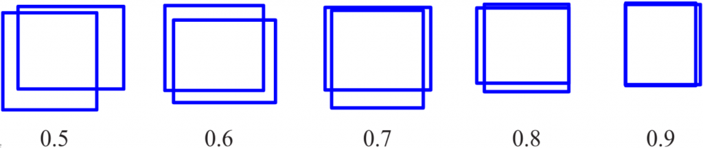
For that, the metric called IoU is used (short for Intersection over Union). We have two bounding boxes: Our prediction and the ground truth bounding box from the training/test set. If our prediction is halfway decent, those bounding boxes should be overlapping somehow. Basically, IoU is a ratio between the intersection area and the union area of the two bounding boxes. The higher the IoU, the more they overlap and the better the prediction. Common practice is to count a prediction as positive if the IoU value is above 0.5.

The anatomy of an object detection network

Most of the recent object detection networks are structured in a very similar way. The term anatomy can be taken quite literally in this case because object detection networks generally consist of a backbone and a head.

The backbone network

The backbone network is the first stage in an object detection network and is responsible for learning the visual features in an image. One could think of its function as “learning to understand images”. These backbone networks are often repurposed CNNs that were actually designed and trained for the image recognition task. The only important thing that is changed is that the last few fully connected layers (the classification layers) are removed so that the feature maps from the convolutional layers can be processed by our new network. By employing these image recognition networks for object detection, we are taking advantage of the fact that these image recognition networks have already learned how to parse and understand an image. The act of transferring a model from one domain to another is known as transfer learning and is very common in NLP (e.g. BERT [18]). As long as the implementational technicalities (such as output format and dimensions) are compatible with the next stage of the model, one should theoretically be able to employ any classification network as a backbone for object detection. With that said, of course the better the backbone, the more capable it is of extracting representational features out of an image.

The detection head

After the image has been processed by the backbone, the detection head is responsible for the actual detection process; identify objects in an image, localize them with bounding boxes and classify them. This is where most of the object detection models will differ from another and we’ll have a look at how some of the most promising models lately go about approaching this task.

Two-stage object detection

Two paradigms have established themselves in object detection: Two-stage models and one-stage models. Arguably one of the most influential two-stage object detection approach is that of the R-CNN family of networks. While they by themselves are not the state-of-the-art anymore, they have built the foundation for one of the highest performing state-of-the-art models today.

In 2014, R-CNN, short for “Regions with CNN features”, [11] revolutionized object detection and legitimized CNNs for this task. However, R-CNN suffered from slow inference speed. The second revision, called Fast R-CNN [14], addressed that issue basically by reordering operations in the network. The third revision, however, increased inference speed yet again and pushed it into the realm of near real-time object detection.

The R-CNN networks are so called two-stage object detector because they divide the task into two sub-tasks:

• Proposing Regions of Interest (RoIs):
  • Suggestion boxes where in the image there might be an object
• Classification
  • Given a RoI, classify the object in the RoI and draw final bounding boxes around it

Faster R-CNN

What exactly makes Faster R-CNN “faster” than its predecessors is two-fold:

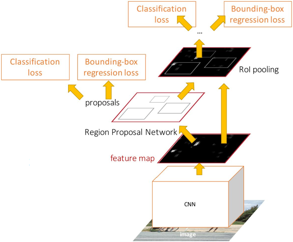
The original R-CNN used to send each RoI through the backbone network individually. This is very slow and inefficient since many region proposals overlap but computation isn’t shared between them. Faster R-CNN, on the other hand, processes the entire image with the backbone in one go before evaluating the region proposals. Because of that, Faster R-CNN shares computation across all RoIs. Once the image has been processed by the backbone, the second improvement picks up.

Both the original R-CNN and the first revision, Fast R-CNN, used a traditional (i.e. not using deep learning), off-the-shelf computer vision method for proposing RoIs. This means the proposal mechanism cannot be learned during training. Faster R-CNN improves on this by introducing a new subpart of the network called the Region Proposal Network (RPN). Now, for the first time, the process of proposing RoIs can be actually learned. This improved speed tremendously, enabling practically real-time object detection with about 0.2s per frame.

The RPN learns two overarching sub-tasks:

• Proposing rough bounding boxes of RoIs (“Where could an object be?”)
• Predicting the “objectness” of RoIs (“How sure am I that there’s an object in here?”)

How does the RPN learn to propose regions of interest?

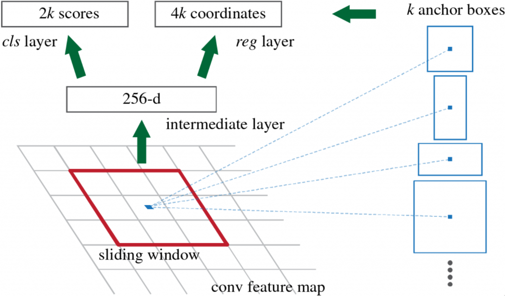
On a high level, it moves so called anchor boxes over the feature map that it got from the backbone network. At each anchor position, it considers nine different boxes with that anchor as their center. These nine boxes are of different scales and aspect ratios. The RPN then builds feature vectors out of the contents of those anchor boxes. Within the RPN, two sibling branches of fully connected layers follow to predict the two aforementioned sub-tasks.

• regression branch: predicts rough bounding boxes of the RoI
• classification branch: predicts the “objectness” of the RoI

After the RPN has found a set of region proposals, those have to be mapped to a fixed-sized shape. This is because the following part of the network, the classifier part that actually predicts the object class, expects feature vectors of a fixed size. To be compatible with the classifier, the feature vectors are mapped to a fixed size by using a method called RoI-Pooling. What RoI-Pooling basically does, is to warp and resize the RoIs (that can be of different size!) into a fixed size.

Once those RoIs have been prepared for the final step, they are then sent to the final part of the entire network that is responsible for the final two sub-tasks:

• Correct the bounding boxes that the RPN has proposed
• Finally predict what kind of object is in the RoI

The act of actually learning and performing the RoI proposals in-house, instead of employing an off-the-shelf algorithm, boosted inference speed to practically real-time (about 0.2s for one test image compared to the 2.3s from Fast R-CNN).

To summarize, the most important factors that make Faster R-CNN so good and efficient are that it

1. shares computation for region proposals
2. actually learns and generates RoI proposals in the same network.

Mask R-CNN [7]

Faster R-CNN got very popular and has even been adopted for instance segmentation. Instead of drawing bounding boxes around objects, the task in instance segmentation is to draw masks over objects as accurately as possible, hence the name Mask R-CNN.

In the context of this write-up, for our intents and purposes Mask R-CNN is basically a Faster R-CNN for object detection but with an extension that allows it to draw the segmentation masks. One key difference between the two, however, is that Faster R-CNN uses RoI-Pooling, while Mask R-CNN uses RoI-Align. To reiterate, RoI-Pooling was done to map different sized RoIs to a fixed size. The problem with RoI-Pooling, though, is that it’s quantized. If we’re unlucky, the pixel area of the input RoI and the pixel area of the target size don’t line up well and we distort the image or lose information in the process. As you can see in the example image of RoI-Pooling, resulting pooled areas are of different size because the RoI has odd dimensions.

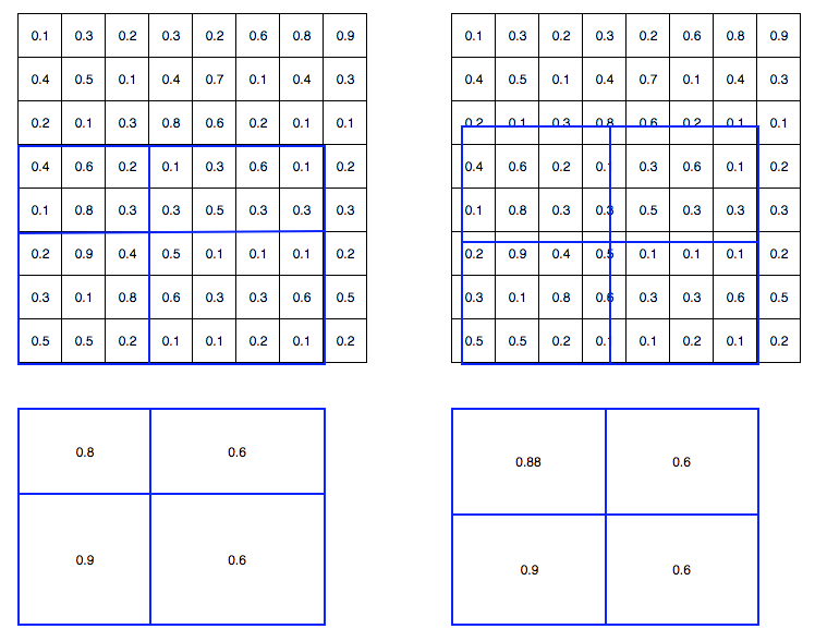
RoI-Align solves that problem by interpolating values in between pixels using bi-linear interpolation. That way, we can obtain fixed-sized vectors without distorting the image or losing information.

Two-stage object detection state-of-the-art:

Cascade R-CNN [3]

The authors of this paper [3] saw the following problems with how object detection has been done up to that point:

Most models, if not all, conventionally defined a bounding box prediction to be positive if the IoU value is above 0.5 (scroll back to the beginning of the page to see what that looks like). The authors hypothesized that the IoU threshold of 0.5 is too low and leads noisy predictions. When a model is trained on such a low IoU, the network will not be able to distinguish good predictions from false positives that are close but not quite correct. In other words, if a model is trained on too low of an IoU, it will fail to reject close false positives. As a result, precision will suffer. What the authors saw, was that performance in object detection seemed to saturate because of that.

Now you might be thinking “Well if training on a low IoU threshold is bad, why don’t they just increase it and get on with it?”
Unfortunately, it isn’t quite that simple. This is what the authors call the paradox of high-quality detection, where “high-quality” stands for the high IoU threshold. It states that training a detector with a higher threshold actually leads to worse performance, not better!
This problem has two causes:

• The RoI proposal mechanisms are biased towards lower quality proposals, meaning they tend to produce proposals with a lower IoU rather than high. If we simply increase the IoU threshold that the detector head demands, the proposal mechanism will just fail to fulfill the expectations and crumbles under the pressure. (You and me both, buddy.) This means that now fewer positive training samples are accepted and the detector head won’t have a lot learn from, which is detrimental for neural networks since they are so reliant on having lots of data
• Even if we did manage to train the detector to a high IoU threshold, we won’t be able to capitalize off of it if, at test time, the region proposals are still bad. The authors observed that the detector head will only perform well if it is provided with good region proposals. It does not fare well out of its comfort zone.

Basically, these two problems boil down to one problem/solution:
We need to make sure that both the RoI proposal method and the detector head are improved at the same time, so that they match in quality and don’t bottleneck one another.

Architecture

Enter: Cascade R-CNN. The architecture is, as the name suggests, very similar to the R-CNN, specifically Faster R-CNN.

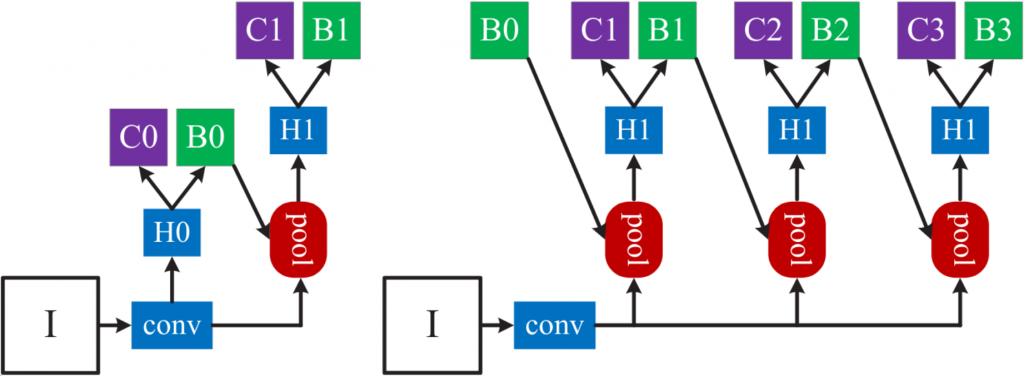
While the R-CNN variations would stop working on an image once the second and final bounding box prediction has been made, Cascade R-CNN will keep those bounding box predictions in the network and further improve on them. By treating the predicted bounding boxes like new RoI proposals, Cascade R-CNN can send those bounding box predictions to the next stage of its cascade and redo the prediction. One stage’s prediction is another stage’s region proposal. It’s easy to see that after each stage, the bounding boxes will iteratively get better and better. By learning with this architecture, each stage in the cascade will actually specialize in a certain IoU area. The first stage will specialize in generating and classifying low-IoU samples, the second stage in mid-tier and the third stage in high-IoU samples. That way, the authors solved the problems mentioned above in one go:

• Detector heads now have access to higher quality region proposals (since they recycle bounding box predictions from the preceding steps and each pass on improved versions)
• Both the quality of region proposals and the specialization of the detector heads now match since they both specialize in a certain IoU range.

This architecture can be applied to any two-stage object detector that is based on R-CNN, which means we can even use Mask R-CNN. This architecture, combined with Mask R-CNN, is aptly called Cascade Mask R-CNN.

CBNet [9]: Composite backbones

Until now, the backbone networks have taken on a relatively minor role in this write-up. To recap, backbone networks are CNNs that extract the features out of the image for the detector head to work with. The more powerful the backbone network, the better it can extract representational features from the image. Backbone networks have mostly been single, repurposed pre-trained networks from the image classification task. That is until CBNet [9] came around and introduced an architecture specifically for object detection.

CBNet, which stands for Composite Backbone Network, is a backbone architecture that makes use of not one but multiple backbones in parallel.

Architecture

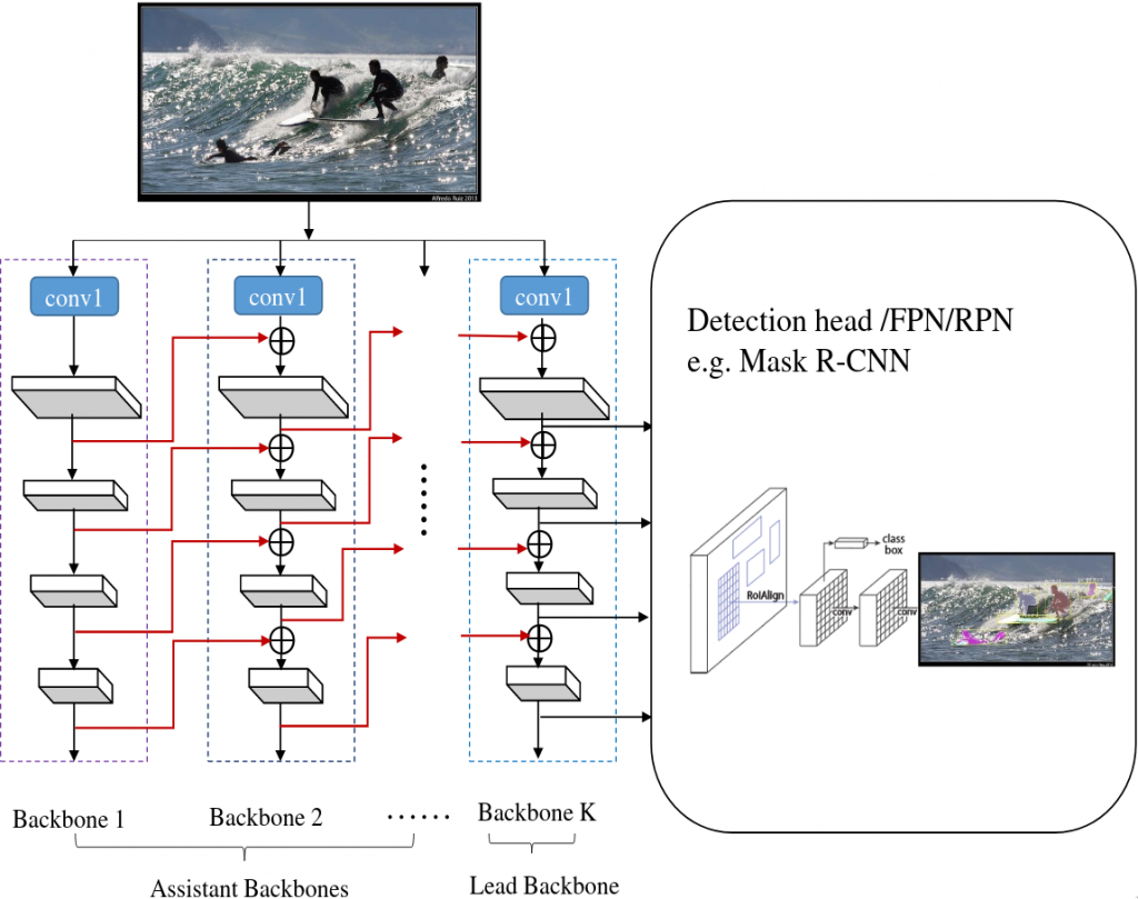
CBNet consists of one or multiple identical assistant backbones and one lead backbone. Each one of these backbones by themselves are normal backbones that have been used by other architectures already, they are pre-trained and readily available. In between the backbones there are so called composite connections. In the main implementation, these composite connections route the output of each stage in the first backbone as input to the parallel stage in the second backbone one level higher. This particular configuration is called AHLC, short for Adjacent Higher Level Composition. It’s done to fuse features of higher levels and scales with features of lower levels/scales to get richer representations than if the backbones and their levels were on their own and not communicating. After traversing through the assistant backbone(s), you reach the lead backbone which will return the final features for the detection head to digest.

For the detection head, you should be able to use any object detector that expects a backbone output, such as the R-CNN variants, Mask R-CNN and Cascade Mask R-CNN.

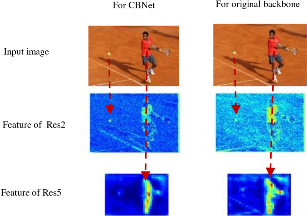
The authors have tried other composite connection configurations, such as Adjacent Lower-Level Composition (ALLC), where instead of fusing the output of one layer with the adjacent higher level output, you fuse it with the one below the parallel level. Another configuration the authors have tried is the same-level configuration. After evaluating and comparing the configurations, however, they found that the higher-level configuration was the only one to improve performance but it did so significantly. Analysis showed that the right kind of composite connections are the crucial part of the network that increased performance. As a result, object detectors using CBNet are able to pay more attention to foreground objects.

The ultimate combination:
Cascade Mask R-CNN with CBNet backbones

The combination of these last 3 models, (Cascade Mask R-CNN with a triple ResNeXt152 backbone à la CBNet) resulted in the current state-of-the-art model that has yet to be beaten in performance since September 2019 (as of May 2020) [9] [10]. While this combination performs really well on the precision side of things, inference time isn’t its main focus. Even though it’s a descendant of a model whose name is literally “Faster R-CNN” and promises practically real-time object detection, the state-of-the-art model’s strength lies in its high performance.

---

If your goal is to have good enough object detection that has a high number of frames per second, there are other, faster options.

Why should I care about faster object detection?
The obvious use case would be autonomous driving, where frames can mean the difference between life and death, especially at high speeds.

Okay, but why would I care as a computational linguist?
Yes, maybe we computational linguists would probably prioritize accuracy over speed for our use cases. However, the following state-of-the-art-model also has other redeeming traits that will come in handy for anyone who wants to do object detection on their own.

---

One-stage object detection:
YOLO

Unlike the R-CNN variants described above, YOLO is considered a one-stage object detection architecture. Two-stage architectures first propose RoIs of varying sizes, then run a classifier over all those regions. This means the model looks at the image multiple times in order to perform object detection on the image. YOLO, which in this case stands for “You Only Look Once”, aims to do all of that in just one go, which the authors call “unified detection”. Instead of proposing rough regions and then refining the bounding boxes, YOLO looks at the image once and regresses the bounding boxes right away. One advantage YOLO has because of this is that it sees the entire image and thus learns contextual information in the image as well. The previously discussed two-stage methods don’t do that because they regard each RoI individually. Because of this, the R-CNN variants produce more false positives compared to YOLO, meaning they falsely classify background as an object. If they had more information about the big picture (no pun intended), they wouldn’t be so quick to classify a patch of background as an object.

YOLO has seen many revisions, with the fourth one being released just end of April 2020.

YOLOv1 [12]

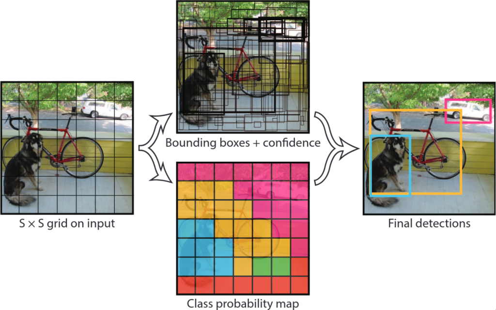
YOLO regards object detection not as a classification task but a regression task. One single network predicts multiple bounding boxes and class probabilities of those bounding boxes, all at once.

The input image is divided into grid cells. Each grid cell will then predict a pre-set number of bounding boxes and an associated probability p(object) that that bounding box contains an object. These bounding boxes can, and in many cases should, span across multiple grid cells. So far it sounds very similar to the Faster R-CNNs RPN network. The difference, however, lies in the fact that the RPN uses anchor boxes of fixed size and aspect ratio. YOLOv1, on the other hand, directly regresses a bounding box by its center point coordinates, box width and box height.

In addition to the “objectness” score/probability, each grid cell will simultaneously predict the conditional probability of an object class, given that an object is indeed present in the grid cell. So not only does it predict how likely it is for an object to be in that box, it also predicts what class it would probably be if there really is an object there. Out of the possibly many grid cells that the object covers, a single one will then be responsible for classifying the object. During training, the one grid cell that coincides with the center point of the ground truth bounding box is the one to do it. At inference time, of course, there aren’t any ground truth bounding boxes. More often than not, it’s often clear which grid cell coincides with the center of an object. However, when the object is large and multiple bounding boxes from different grid cells overlap a lot and try to predict the same object, the bounding box with the highest class probability is picked (in a process called non-maximum suppression). That way, we only have one bounding box for one object.

To train the classification and obtain the probability of a class i in a particular bounding box, we multiply the two probabilities and the IoU score of the predicted bounding box and the ground truth bounding box

$$p(\text{class}_i | \text{object}) \cdot p(\text{object}) \cdot \text{IoU} = p(\text{class}_i) \cdot \text{IoU}$$

By multiplying the probabilities with the IoU, this score encapsulates both the class probability and how well the bounding box fits the ground truth.

YOLO is realized as a conceptually relatively simple CNN consisting of multiple common convolutional layers for feature extraction and a few fully connected layers for predicting scores and bounding box coordinates.

Limitations

YOLOv1 has limitations, some of which were addressed in versions 2 and 3. The following problem is one of the limitations that were addressed by YOLOv4. Bounding box coordinates errors are quantified by squared errors in the loss function. This means that errors are weighted the same in absolute terms, regardless of how large the bounding box is. The same absolute difference in, say, bounding box width has a lot more impact on the IoU if the bounding box is small. In relative terms, when considering one particular IoU value, the absolute difference in the coordinates is higher at larger scales than it is at smaller scales.

YOLOv4 [13]

YOLOv4 is the fourth iteration of this object detector family. The new improvements that YOLOv4 brings are its hugely improved performance while maintaining the high frame rate that makes YOLO so great.

YOLOv4 improves performance not by overhauling the architecture like Fast(er) R-CNN did with the original. Instead, YOLOv4 optimizes performance by a smart selection of network components and design choices. The authors separate those into two groups: Bag of freebies and bag of specials.

Bag of freebies

By bag of freebies, the authors describe methods that only change the training strategy or increase the training cost, which means they come at no cost to inference. One such example we know from computational linguistics, too, is data augmentation. Data augmentation serves to prevent overfitting and make the model generalize better. Other freebies include methods for overcoming imbalance between the classes in the training data. To address the aforementioned problem of the bounding box error, YOLOv4 considers other loss functions using the bounding box IoU instead of the bounding box coordinates.

Bag of specials

The bag of specials on the other hand contains methods and post processing that increase inference cost by a little but greatly improve accuracy. These are for enhancing certain properties of a model such as “enlarging receptive field and introducing attention mechanism” among others [14]. The use and choice of a non-maximum suppression method (for removing duplicate bounding boxes) also falls into this category.

Additional improvements

One of the most attractive improvements of YOLOv4 for us computational linguists is the fact that now it can be trained on a single consumer-grade GPU. This is achieved through some additional improvements the authors made.

Two new data augmentation techniques are introduced: mosaic and self-adversarial training. Mosaic is a technique to merge four training images together in a mosaic to paste objects into new, unusual visual contexts in which they’re not necessarily found normally. Self-adversarial training is a technique to alter the image in such a way that would fool the model into thinking that there is no object present in the image. The model then has to perform object detection on that image as if it were like any other. These novel methods, combined with modifications to existing methods and an optimal choice of hyperparameters, elevate YOLO to a stage where it can be trained and tested on a consumer grade GPU.
For a more detailed list and explanation on the many specific methods, options and modifications, please refer to the paper [13].

Summary of the state-of-the-art

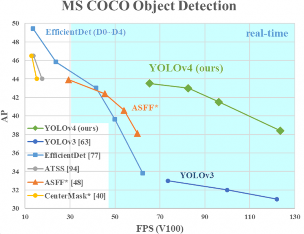
The collection of the many improvements for YOLO have lead to new heights in performance for real-time object detection and even rival many of the models designed for non-real-time high-quality detection. Because of that, YOLOv4 seems to be the closest thing to a no-compromise solution for object detection that we have right now.

If, however, performance your top priority, there are still other models which produce higher scores. The one to be at the top of the high-quality models currently seems to be Cascade Mask R-CNN with a composite backbone, embodying the combined effort of optimized backbone architecture, production of high-quality region proposals and conjunction with high-quality classification.

Related models and honorable mentions

While YOLOv4 is unrivaled in high-speed object detection by a huge margin (to be fair, it hasn’t been out for a long time yet), there are other one-stage object detectors such as SSD (Single Shot Multibox Detector) [15] that are also well known.

Meanwhile, competition at the high-performance end of the spectrum is tough. It is true that Cascade Mask R-CNN has been at the top of the game. However, a new backbone proposed at the end of April 2020 (ResNeSt-200DCN) has shown to slightly improve object detection performance yet again compared to the previously used backbone. In terms of other competitor architecture, the fight between Cascade Mask R-CNN and the EfficientDet-D7 [16] network is almost a toss-up at the moment, as their detection scores are very very close.

Conclusion

Object detection is a very active field that is seeing a lot of optimization and innovation. With the advent of autonomous driving, the demand for good and fast object detection is at an all time high. As computational linguists, our most immediate concern might not be speed but rather performance, at least for now, especially in scenarios where we have to predict one correct label out of very many (the entire English vocabulary). Furthermore, in scenarios such as phrase grounding, it would be very useful to be able to predict multiple labels as well, for example recognizing and understanding that a woman is also a person and a human. So while detection speed might not be the most attractive feature to us, the ongoing progress in portability and accessibility can still greatly enhance our experience when trying to employ object detection for multimodal tasks. With interesting ideas in zero shot learning for the future, and applications in AI assistants, object detection and multimodality will only become more relevant as technology improves and time goes on.

---

References

1. Malhotra, S. (2020) What is zero shot learning? https://www.quora.com/What-is-zero-shot-learning
2. Alibaba Tech. (2018). From Zero to Hero: Shaking Up the Field of Zero-shot Learning. https://medium.com/@alitech_2017/from-zero-to-hero-shaking-up-the-field-of-zero-shot-learning-c43208f71332
3. Cai, Z., & Vasconcelos, N. (2019). Cascade R-CNN: High quality object detection and instance segmentation. IEEE Transactions on Pattern Analysis and Machine Intelligence.
4. Ren, S., He, K., Girshick, R., & Sun, J. (2015). Faster R-CNN: Towards real-time object detection with region proposal networks. In Advances in neural information processing systems (pp. 91-99).
5. Fei-Fei Li, Justin Johnson, and Serena Yeung (2017). Lecture 11 — Detection and Segmentation. https://youtu.be/nDPWywWRIRo.
6. Grel, T. (2017). Regions of interest pooling explained. https://deepsense.ai/region-of-interest-pooling-explained/
7. He, K., Gkioxari, G., Dollár, P., & Girshick, R. (2017). Mask R-CNN. In Proceedings of the IEEE international conference on computer vision (pp. 2961-2969).
8. Hui, J. (2018). Image segmentation with Mask R-CNN. https://towardsdatascience.com/understanding-region-of-interest-part-2-roi-align-and-roi-warp-f795196fc193
9. Liu, Y., Wang, Y., Wang, S., Liang, T., Zhao, Q., Tang, Z., & Ling, H. (2019). CBNet: A novel composite backbone network architecture for object detection. arXiv preprint arXiv:1909.03625.
10. https://paperswithcode.com/task/object-detection (Last accessed: May 17, 2020)
11. Girshick, R., Donahue, J., Darrell, T., & Malik, J. (2014). Rich feature hierarchies for accurate object detection and semantic segmentation. In Proceedings of the IEEE conference on computer vision and pattern recognition (pp. 580-587).
12. Redmon, J., Divvala, S., Girshick, R., & Farhadi, A. (2016). You only look once: Unified, real-time object detection. In Proceedings of the IEEE conference on computer vision and pattern recognition (pp. 779-788).
13. Bochkovskiy, A., Wang, C. Y., & Liao, H. Y. M. (2020). YOLOv4: Optimal Speed and Accuracy of Object Detection. arXiv preprint arXiv:2004.10934.
14. Girshick, R. (2015). Fast r-cnn. In Proceedings of the IEEE international conference on computer vision (pp. 1440-1448).
15. Liu, W., Anguelov, D., Erhan, D., Szegedy, C., Reed, S., Fu, C. Y., & Berg, A. C. (2016, October). Ssd: Single shot multibox detector. In European conference on computer vision (pp. 21-37). Springer, Cham.
16. Tan, M., Pang, R., & Le, Q. V. (2019). Efficientdet: Scalable and efficient object detection. arXiv preprint arXiv:1911.09070.
17. Yang, Z., Zhang, Y. J., Rehman, S. U., Huang, Y. (2017). Image captioning with object detection and localization. arXiv preprint arXiv:170.024
18. Devlin, J., Chang, M. W., Lee, K., Toutanova, K., (2018). Bert: Pre-training of deep bidirectional transformers for language understanding.